Monte Carlo for Options Sellers: Simulating Assignment Risk and Income Before You Trade
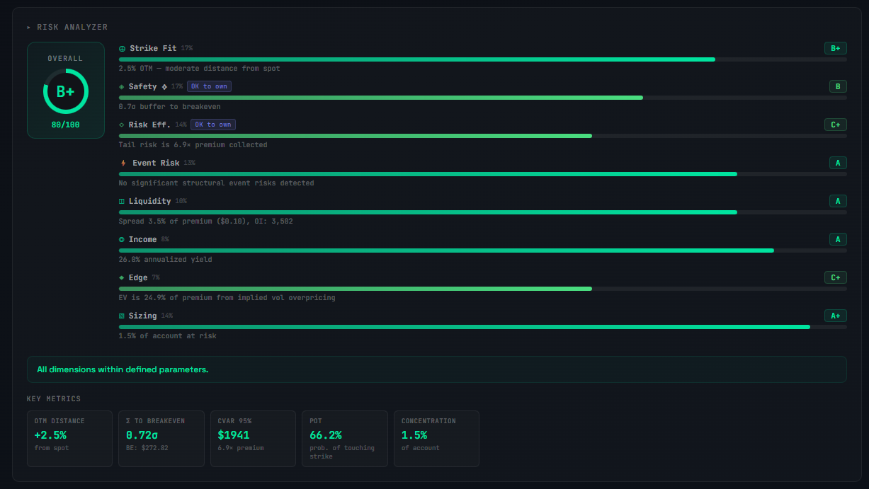
You've found a setup that looks good. The delta is in range, the premium yield is solid, the spread is tight. The grading system gives it a B+. You're ready to sell.
But there's a question the grade doesn't answer: what's the actual probability that this trade ends with you keeping the premium versus getting assigned?
And if you repeat this kind of trade every month, what does your income look like over a year — accounting for the cycles where things don't go to plan?
Delta gives you a rough approximation. A 0.25 delta put has roughly a 25% chance of finishing in the money. But delta is a snapshot — it assumes constant volatility and a single point in time.
Real stocks gap, trend, and cluster their moves. The actual distribution of outcomes is messier than delta implies.
This is where Monte Carlo simulation earns its place in the toolkit.
What Monte Carlo Simulation Actually Does
Monte Carlo is a brute-force approach to probability. Instead of solving a formula for the "correct" answer, you simulate thousands of possible futures and count the results.
For an options seller, it works like this:
- Take the current stock price, implied volatility, and time to expiration.
- Generate a random price path — a series of daily moves based on the stock's volatility.
- Check where the stock lands at expiration. Is it above or below your strike?
- Repeat thousands of times.
- Count how many paths ended with you keeping premium versus getting assigned.
The result isn't a single number — it's a distribution.
You don't get "there's a 23% chance of assignment." You get a full picture: 7,400 paths where you kept premium, 2,600 where you got assigned, and the spread of outcomes within each bucket.
That distribution tells you more than delta ever could.
Under the Hood: The Random Walk
Each simulated price path follows a model called Geometric Brownian Motion. In plain language: the stock moves up or down each day by a random amount, scaled by its implied volatility.
Higher IV means wider daily moves and a wider fan of possible outcomes. Lower IV means the paths stay tighter.
The simulation uses the stock's current implied volatility as its input, so the paths you see reflect what the market is actually pricing in right now — not some historical average.
Each daily step looks like this: take yesterday's price, apply a small drift (the risk-free rate), then add a random shock scaled by volatility. Repeat for every day until expiration. At the end, check if the stock finished above or below your strike.
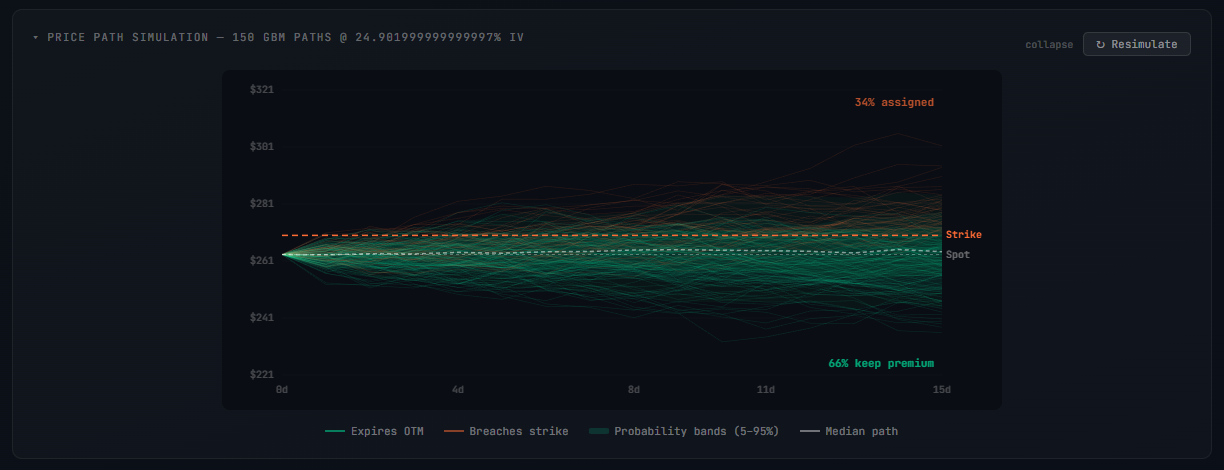
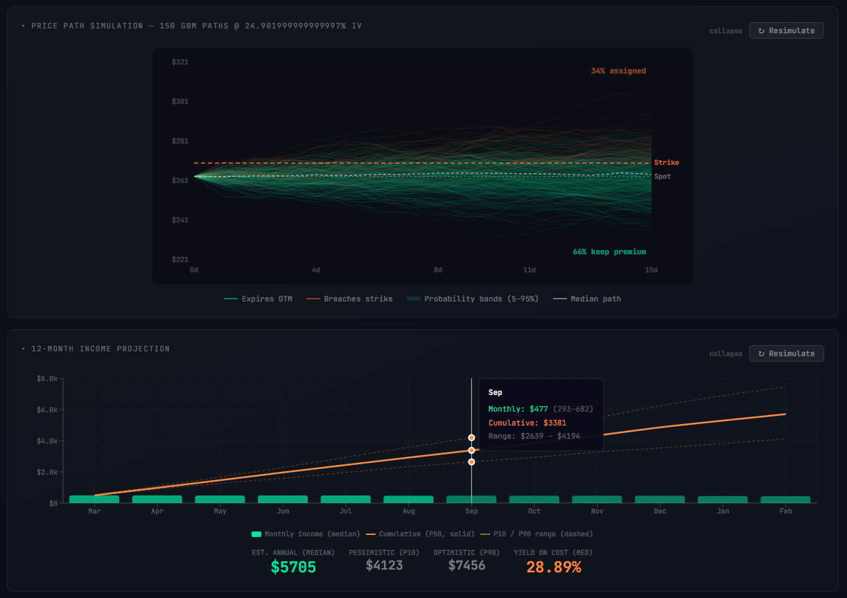
Run that 150 times and you get a visual fan of price paths. The paths that end beyond your strike light up orange — those are assignment scenarios. The paths that stay safe are green — you keep the premium.
The simulation also extracts percentile bands across all paths: the 5th, 25th, 50th (median), 75th, and 95th percentiles at each point in time. These bands show you the likely range of outcomes and how wide the uncertainty is at any point during the trade.
Why Delta Isn't Enough
Delta comes from the Black-Scholes model, which assumes stock prices follow a neat statistical distribution with constant volatility. That's a useful simplification, but it misses things that matter:
Volatility isn't constant. IV can spike or compress between now and expiration. A 0.25 delta put today might behave like a 0.35 delta put next week if volatility expands.
Returns have fat tails. Real stocks make extreme moves more often than the standard model predicts. This is the exact risk options sellers need to worry about most — the gap down that blows through your strike.
Path matters. Delta tells you about the endpoint. It says nothing about whether the stock gapped down 15% mid-cycle before recovering. If you're managing positions actively, the path changes your decisions.
Monte Carlo doesn't solve all of these perfectly, but by simulating hundreds of possible paths, it captures the range of outcomes in a way that a single Greek value can't.
How Intent Changes Everything
Before running any simulation, you set a trade intent: Avoid Assignment or OK With Assignment.
This single toggle transforms the entire analysis — not just the strike selection, but how the simulation calculates your P&L across every path.
Avoid Assignment
You want to keep your shares (covered calls) or keep your cash (puts) and just collect premium. The engine steers toward lower-delta, further OTM strikes.
Here's the critical part: when the simulation encounters an assignment scenario on an "avoid" intent, it models the cost of getting out.
In real trading, if you're assigned against your intent, you'd roll the position or close early — and that costs money. The simulation applies a penalty: you lose a portion of the intrinsic value the option went against you, modeling the real-world cost of rolling out for a credit.
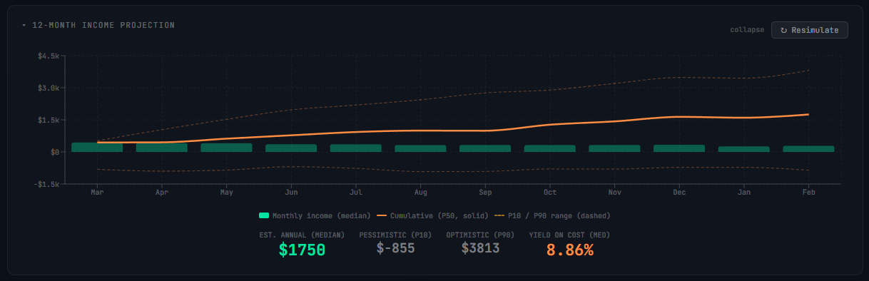
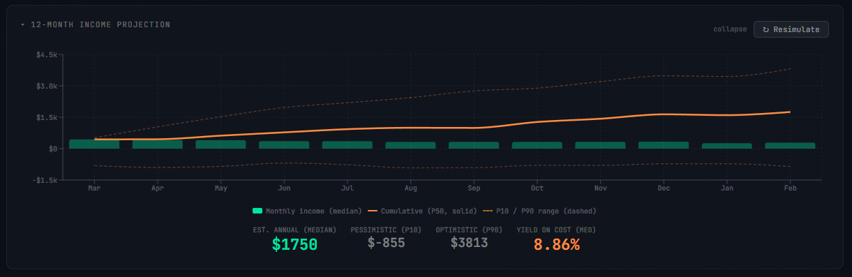
This means the "avoid assignment" simulation can and will produce negative months. If a simulated path drops hard through your strike, the penalty for rolling or closing at a loss can exceed the premium you collected that cycle.
Over 12 months, some paths will show months where your income goes red.
That's not a bug — it's reality. If you're selling with the intent to avoid assignment, the months where assignment happens anyway are expensive. The simulation shows you exactly how expensive, and how often.
OK With Assignment
You're willing to buy the shares (puts) or sell them (calls). The engine opens up higher-delta, closer-to-the-money strikes with richer premiums.
When assignment happens here, there's no penalty. You wanted the shares — you keep the full premium and move on to the next phase (selling covered calls against your new position, or selling puts again after your shares are called away).
The assignment isn't a loss; it's part of the plan.
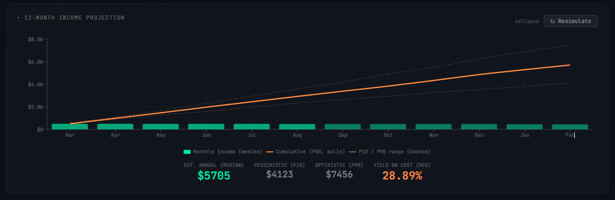
This means the "OK with assignment" projection is smoother and almost always positive month-to-month. You're collecting fatter premiums with higher assignment probability, but assignment doesn't hurt because it's the intended outcome.
The Difference Is Dramatic
Run the same ticker, same expiration, same delta on both intents and the 12-month projections look completely different:
Avoid assignment — lower premium per cycle, some negative months from rolling costs, but more cycles completed because you're rarely locked into an assigned position. The median annual income might be similar, but the P10 (worst case) band dips below zero in some months.
OK with assignment — higher premium per cycle, no negative months from assignment, but fewer pure premium cycles because some months are spent in the covered call phase working out of an assigned position. Smoother curve, tighter confidence bands.
Neither is better. They're different strategies for different goals. The simulation makes the tradeoff visible instead of theoretical.
The 12-Month Income Projection
The single-trade Monte Carlo shows you one cycle. The 12-month projection answers the bigger question: what does this strategy produce over a year?
This is a separate, more sophisticated simulation. It runs 200 paths across 12 months, and it introduces something the single-trade simulation doesn't: correlated spot and volatility dynamics.
Why Spot and IV Move Together
In reality, stock prices and implied volatility aren't independent. When a stock sells off, IV tends to spike. When it rallies, IV tends to compress.
This is called the leverage effect, and it's one of the most consistent patterns in options markets.
The income projection models this directly. Each simulated path evolves both the stock price and its implied volatility simultaneously, with a negative correlation between them.
When the simulated stock drops, simulated IV rises — which means the next cycle's premium is richer, but the assignment risk is also higher.
This is important because it captures a real dynamic that flat models miss: bad months (where you get assigned) tend to be followed by months with elevated premium (because IV spiked). And good months (premium collected, stock calm) tend to be followed by periods of thinner premiums (because IV compressed).
The projection reflects this push-pull instead of assuming every month looks the same.
IV Itself Fluctuates
The model doesn't just correlate IV with spot — it lets IV wander on its own too.
Implied volatility tends to mean-revert: when it spikes, it eventually drifts back down. When it compresses, it eventually picks back up. The projection models this with a mean-reverting process, where IV is pulled back toward its current level over time but with its own randomness layered on top.
This means some simulated paths experience a sustained low-IV environment (thin premiums for months) while others experience a vol spike followed by gradual normalization.
The spread of these IV paths is what creates the width of the confidence bands in the projection chart.
Dynamic Strike Selection
Each simulated cycle doesn't use a fixed strike. As the simulated stock price and IV evolve month to month, the engine re-selects the appropriate strike for each new cycle based on your target delta.
If the simulated stock has dropped 10% and IV has spiked, the engine picks a strike further OTM with richer premium — just like a real trader would adapt. If the stock has rallied and IV has compressed, the strike adjusts accordingly.
This makes the projection realistic. It's not assuming you sell the same $45 put every month for a year. It's modeling how your actual strike selection would shift as conditions change.
Reading the Output
The projection chart shows cumulative income across 12 months with confidence bands:
P50 (median) — the middle path. Half of simulated outcomes are above this, half below. This is your "expected" annual income from the strategy.
P10 and P90 — the 80% confidence range. In 80% of simulations, your annual income falls within this band. The wider the band, the more uncertain the outcome.
P25 and P75 — the tighter 50% range. More probable outcomes live here.
If the P10 line dips negative in certain months (common with "avoid assignment" intent), that tells you there are realistic scenarios where your strategy loses money in the short term before recovering.
If the P10 stays positive throughout, the strategy is robust across most market conditions.
Putting Risk and Income Together
The power of combining Monte Carlo assignment analysis with income projections is that you see both sides of the trade:
What could go wrong — the assignment probability, the tail risk, the worst-case scenarios across thousands of paths.
What you're building toward — the cumulative income over 12 months if you execute the strategy consistently, with realistic modeling of how spot and volatility interact.
This changes how you evaluate individual setups. A trade with a slightly lower grade but better tail risk might project higher 12-month income than a higher-yielding setup that occasionally blows up. The simulation makes this visible.
It also helps with position sizing. If the Monte Carlo shows a 5% chance of a 20%+ drawdown on assignment, you can size the position so that worst case doesn't damage your portfolio.
If the 12-month projection shows the P10 band going negative in month 3, you know to keep reserves for that scenario.
How to Use This in Practice
Before entering any cash-secured put or covered call:
Set your intent first. This isn't a toggle you flip after the fact — it drives the entire analysis. Know whether you're optimizing for premium collection (avoid assignment) or the full wheel cycle (OK with assignment) before you look at any numbers.
Run the simulation. Compare the Monte Carlo assignment probability against delta. If they diverge, understand why. Elevated IV and fat tails can push assignment probability higher than delta suggests.
Check the tails. What does the worst 5% of outcomes look like? Can you live with that scenario at your current position size?
Look at the 12-month projection. Does the median annual income justify the capital commitment? Is the P10 band acceptable, or does it show months of drawdown you can't stomach?
Compare intents. Run both "avoid" and "OK with assignment" on the same setup. The difference in projected income and risk profile might change which approach you take.
The simulation doesn't replace judgment. But it replaces the part of judgment that humans are worst at — estimating probabilities and compound outcomes over time.
Try It Yourself
The RISK tab in ThetaHarvester runs Monte Carlo simulations on your selected setup with real-time options data. It shows assignment versus keep-premium probabilities, outcome distribution bands, and a 12-month income projection with correlated spot-IV dynamics.
Toggle between "Avoid Assignment" and "OK With Assignment" and watch the entire projection shift — the strike selection, the premium per cycle, the confidence bands, and the months where income dips negative.
Free users can explore the full tool using demo tickers (AAPL, SPY, TSLA, NVDA, QQQ, MSFT). No signup form — just a magic link to your email.