Reverse DCF Explained — What Growth Does the Price Imply?

Short answer: A reverse DCF takes the current enterprise value as given and solves for the free cash flow growth rate that justifies it — turning 'the shares look expensive' into 'the price requires 22% growth every year for a decade.' It is the most useful of the four valuation methods because its output is a testable claim, not an opinion. Compare the implied growth rate against what the company actually delivered over the last five years and what its industry is growing at, and you know exactly what you are betting on.

A company is worth the cash it will produce for its owners over its life, converted into today's money. Every share price is therefore a claim about future cash flow — and a reverse DCF is the tool that reads the claim out loud.

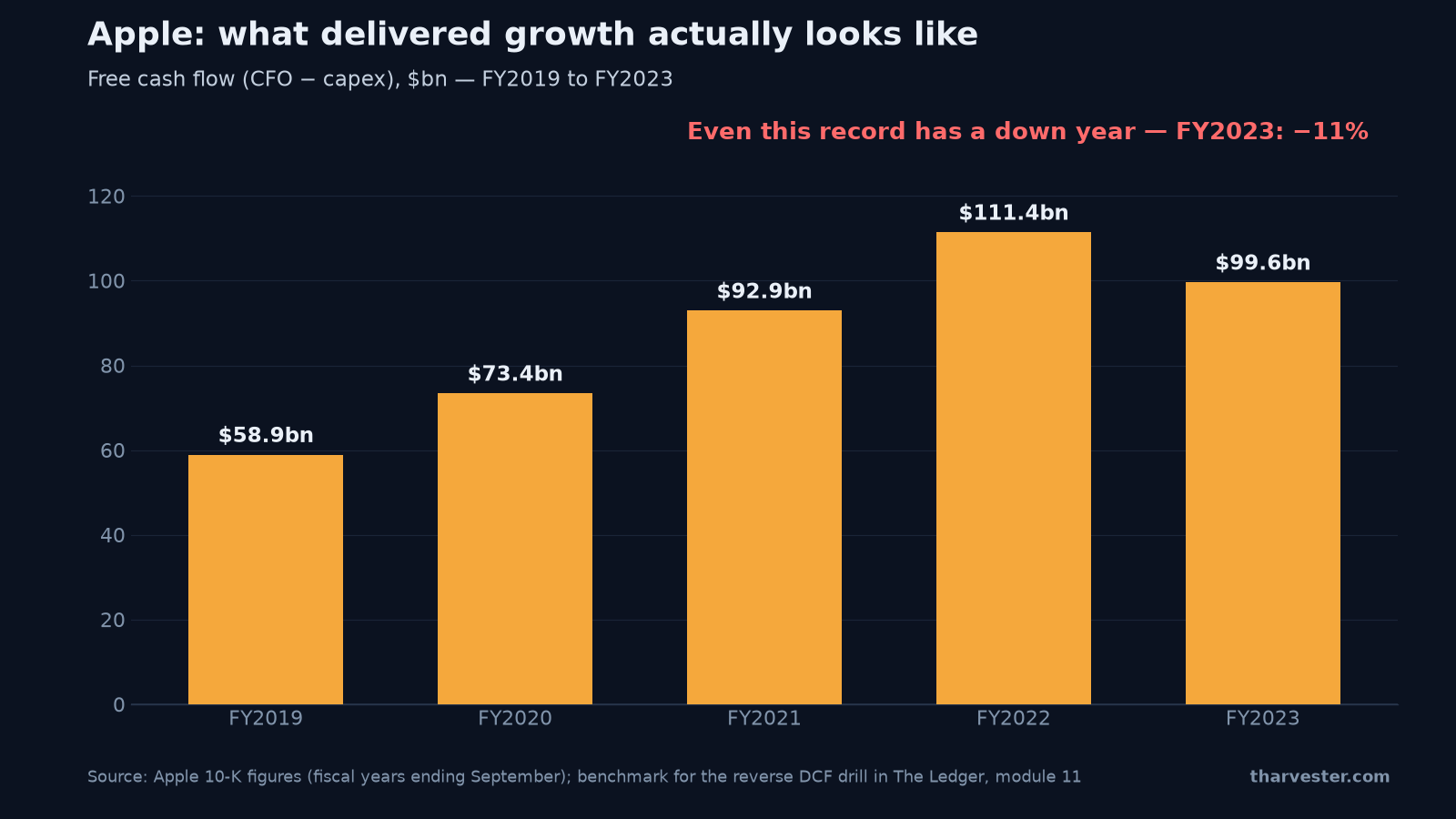
The chart above shows why the reading needs a reality check. It plots Apple's free cash flow — cash from operations minus capital spending — by fiscal year: $58.9bn in FY2019 rising to $111.4bn in FY2022, then falling to $99.6bn in FY2023. Even the largest cash machine in corporate history does not grow in a straight line. Whatever growth rate a price implies, it has to survive years like that. This is module 11 of The Ledger: four valuation methods, used together, because any one on its own is a way to be confidently wrong.

The four valuation methods, and why you need all of them

Method 1 — compare. Take the company's own ratios over the last ten years and see where today sits in that range, then ask what was true at each extreme: was the business genuinely better, or was the market simply more hopeful? Then build a genuine peer set — same end market, same capital intensity, same growth profile — and calculate the ratios yourself on identical definitions, because two data providers will happily give you two different EBITDA figures for the same company. The multiples article earlier in this series covers the ratios themselves; the Ratio Bench computes them all from one set of inputs.

Method 2 — forecast and discount. Method 3 — run it backwards. Method 4 — value the assets, or ask what a buyer would pay. The rest of this article works through the last three.

How a DCF works — and where its value actually comes from

A discounted cash flow (DCF) forecasts free cash flow for the next five to ten years, adds a value for everything after that, and converts the whole lot into today's money. The conversion is the unfamiliar part: money in the future is worth less than money today, because today's money can be invested. If your required return is 9%, then $109 received in a year is worth $109 ÷ 1.09 = $100 today. Cash two years out is divided by 1.09 twice, and so on.

Everything beyond the forecast is compressed into the terminal value:

terminal value = final year cash flow × (1 + g) ÷ (r − g)

where r is the discount rate and g is the growth rate assumed to continue for ever. Now watch where the answer comes from, using the module's worked figures: free cash flow of $450m, growing 5% a year for ten years, discounted at 9%, with 2.5% perpetual growth afterwards.

• Year 10 cash flow: ~$733m (450 × 1.05¹⁰)
• Terminal value at year 10: ~$11,554m (733 × 1.025 ÷ (0.09 − 0.025))
• Terminal value, discounted: ~$4,880m (÷ 1.09¹⁰)
• Share of total value from the terminal: ~63%

Around 63% of the answer comes from the assumption about what happens after year ten — a period nobody can forecast. Change perpetual growth from 2.5% to 3.5% and the terminal value rises by roughly a fifth. This is not a reason to avoid the method. It is a reason to use it for what it is genuinely good at: not the final number, but the sensitivity table that shows which single assumption your conclusion actually depends on.

Reverse DCF: solve for the implied growth rate

The most useful of the four methods flips the question. Instead of asking what the company is worth, ask: what would have to happen for today's price to be correct?

A reverse DCF takes the current enterprise value as given and solves for the growth rate that justifies it. The output is not a valuation — it is a statement of what the market is currently assuming, expressed as a number you can argue with. "The shares look expensive" becomes "the price requires 22% growth every year for a decade, which would make this company larger than its entire addressable market." "The shares look cheap" becomes "the price only requires 3% growth, while the industry itself is growing 6%." Vague debate, made specific.

This is the solver from the course — try it on a real company:

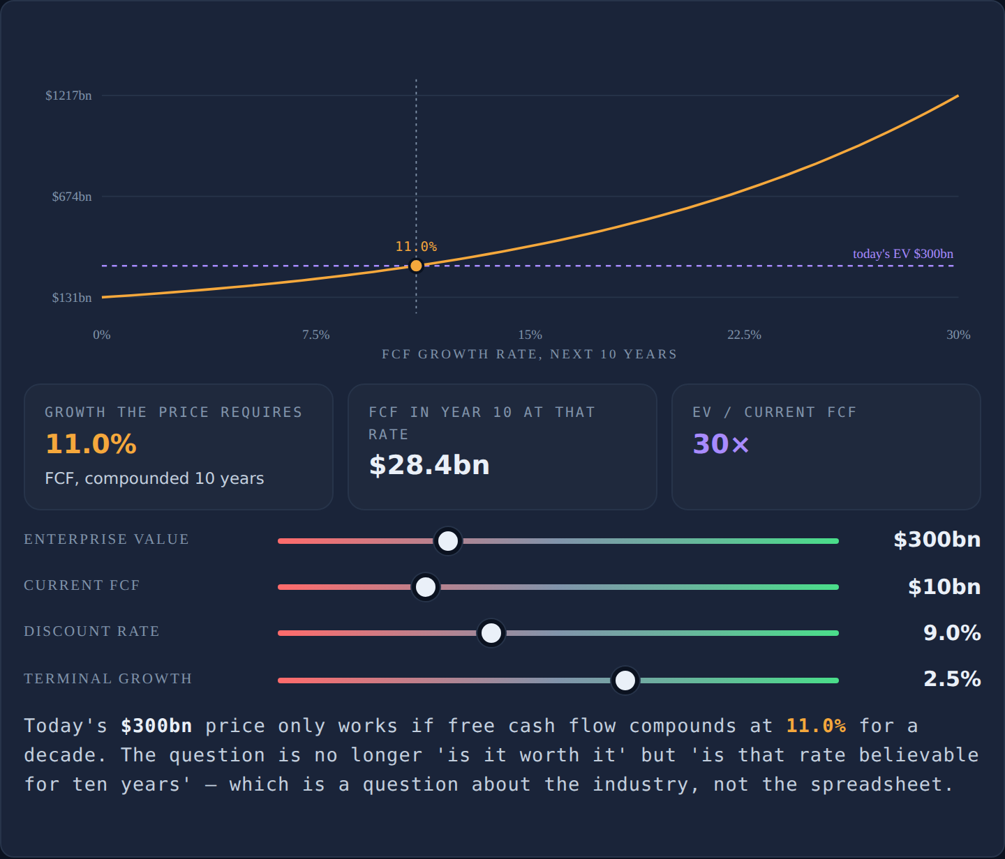
Set enterprise value and current free cash flow for a company you follow, leave the discount rate at 9% and terminal growth at 2.5%, and read the growth rate the price requires over ten years — the chart shows implied value across the whole growth range with a marker at your setting. Then run the sensitivity drill: move only the discount rate, 8% to 9% to 10%, and watch the implied growth swing. That spread is the part of the answer that came from your assumption rather than from the business. Note the tool's honesty at the edges: it refuses, with a reason, when FCF is zero or negative (nothing to grow) or when the discount rate sits at or below terminal growth (the formula implies infinite value).

Test the implied growth against delivered growth

An implied growth rate means nothing in isolation — the module's drill says compare it against two things: what the company actually achieved over the last five years, and what its industry is growing at. That is what the Apple chart at the top is for. FY2019 to FY2023, free cash flow went from $58.9bn to $99.6bn — strong compounding, but with a down year at the end of it. A price that requires a decade of uninterrupted 20% growth is asking for something even businesses of this quality do not reliably deliver. If the price requires more than both the company's record and its industry's growth, you know exactly what you are betting on. If it requires arithmetic impossibility — revenue larger than the addressable market by year ten — you have found something better than an opinion. And if the implied bar looks suspiciously easy to clear, check the earnings quality article from the previous module first: a low bar built on paper profit is no bargain.

Asset values, precedent deals, and a range instead of a number

The fourth family prices what exists rather than what is forecast. Sum of the parts: value each division on its appropriate ratio, subtract net debt and the head office — how a valuable division hides inside a dull group, usually unlocked by a demerger. Replacement cost: trading above the cost of rebuilding the asset base invites competitors to build; trading below it deters them, which is how cycle bottoms are identified. Net asset value: a floor for property, funds, shipping and resources — if the marks are honest. Precedent transactions: what buyers actually paid, read against the interest rates of the time — multiples paid when borrowing was nearly free are not a benchmark for a world where it is not.

Then assemble the output the way the module insists: a range, not a number. Run pessimistic, central and optimistic cases with rough probabilities, and compare the distance to the bad case against the distance to the good one. An investment where the upside is +40% and the downside is −45% is a poor one even if the central case is positive — you are risking more than you stand to gain. The Fundamentals Grader runs a version of this comparison automatically when you grade a ticker.

Keep going

The full lesson — Working out what a business is worth — adds drills on building your own ten-year ratio table, a hand-built peer set, and precedent-deal hunting. It is module 11 of The Ledger, free with no signup; terms live in the glossary. Next in the series, the same toolkit turns bearish: short selling analysis — borrow cost, days to cover and squeeze risk.

Solve for the implied growth rate in module 11 — and find out what the price already believes.

Frequently asked questions

What is a reverse DCF?

A reverse discounted cash flow takes the current enterprise value as given and solves for the growth rate that justifies it, instead of forecasting cash flows to produce a price. The output is not a valuation — it is a statement of what the market is currently assuming, expressed as a number you can argue with. 'Expensive' becomes 'the price requires 22% growth for a decade,' which you can test against the size of the market the company sells into.

How do you calculate the implied growth rate in a stock price?

Take the enterprise value, the current free cash flow, a discount rate (9% is a reasonable default), a perpetual growth rate (around 2.5%), and a forecast period of ten years. Then solve for the single annual FCF growth rate that makes the discounted cash flows sum to the enterprise value. The Ledger's reverse DCF tool does the iteration for you — you supply four inputs and read one output.

Why does terminal value dominate a DCF?

In a typical ten-year DCF, roughly 60–80% of the value comes from the terminal value — the lump representing everything after year ten, calculated as final-year cash flow × (1 + g) ÷ (r − g). In the module's worked example, $450m of FCF growing 5% and discounted at 9% produces a terminal value near $11.6bn, about 63% of the total. Most of the answer rests on a period nobody can forecast, which is why the sensitivity table matters more than the output number.

What discount rate should you use in a DCF?

Use your estimated cost of capital — 9% is a sensible default for a typical established company if you have not built a better estimate. Then run the model at 8%, 9% and 10% and write down all three answers. The spread between them is the part of the answer that came from your assumption rather than from the business; if it is wide, any single-number valuation is mostly telling you about the analyst's cost of capital.

What are the four main valuation methods?

One: compare the company against its own ten-year ratio range and a genuine peer set calculated on identical definitions. Two: a discounted cash flow, read for its sensitivity table rather than its output. Three: a reverse DCF, which solves for the growth the price implies. Four: asset-based methods — sum of the parts, replacement cost, net asset value, and precedent transactions. Each is wrong in a different direction, which is exactly why you use them together.

What is sum-of-the-parts valuation?

Value each division on the ratio appropriate to it, add them up, then subtract net debt and the cost of the head office. It is how you find a valuable division hidden inside a dull group — and the event that unlocks the value is usually a demerger. Without an unlocking event, a sum-of-the-parts discount can persist indefinitely.

When does a reverse DCF not work?

Two input combinations produce no meaningful answer. If free cash flow is negative there is nothing to grow, so the calculation is meaningless — model the path back to positive cash flow explicitly instead. And if the discount rate is at or below the perpetual growth rate, the terminal value formula divides by zero or a negative number, implying infinite value. A good tool refuses and says why rather than printing a figure.

Are precedent transactions a reliable valuation benchmark?

Only when read against the credit environment they happened in. A multiple paid when borrowing was nearly free is not a benchmark for a world where debt costs 6%, and quietly using one as if it were is a common way to talk yourself into overpaying. Always note the year of the deal alongside the multiple paid.